José Sabater

We continue our journey , this time we will add complexity to the dataset.

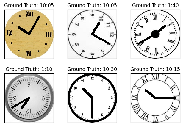
In previous posts we have used mostly the GNIST dataset, containing digits from 0-9. Browsing through Kaggle datasets I found one that I thought could be interesting for classification, and no it´s not the typical cats vs dogs. The dataset has 144 time classes and is all about classifying the correct time. You can find the dataset here.

In this post we will introduce three things one is the handling of datasets, and reading images and the third is how to use the GPU to train your models.

The dataset comes already divided in training , validation and test sets. And everything is mapped in a csv file. We just need to create some loops to handle the information, so we match the correct image with the correct label. In this instance, I created a data frame which I read all the information from.

Length of train_images: 11520
Length of val_images: 1440
Length of test_images: 1440

df = pd.read_csv("../data/time/clocks.csv")
df.head()

	class index	filepaths	labels	data set
0	0	train/1-00/0.jpg	1_00	train
1	0	train/1-00/1.jpg	1_00	train
2	0	train/1-00/11.jpg	1_00	train
3	0	train/1-00/12.jpg	1_00	train
4	0	train/1-00/13.jpg	1_00	train

train_files = df[df["data set"] == "train"]["filepaths"]
val_files = df[df["data set"] == "valid"]["filepaths"]
test_files = df[df["data set"] == "test"]["filepaths"]

train_labels = df[df["data set"] == "train"]["class index"]
val_labels = df[df["data set"] == "valid"]["class index"]
test_labels = df[df["data set"] == "test"]["class index"]

To read the images I did some experimenting of which method was fastest, and I found a very nice benchmark on this GitHub thread. For this post, I will use Pillow but I will leave here two other methods to load the images that are also valid:

# in our dataset 60s
def cv2_imread(path: str) -> np.ndarray:
    img = cv2.imread(path)
    try:
        img = cv2.cvtColor(img, cv2.COLOR_BGR2RGB)
    except:
        pass
    return img

def PIL_read(path: str) -> np.ndarray:
    img = Image.open(path)
    img = np.asarray(img)
    return img


# in our dataset 10s
def PILandShrink_read(path: str) -> np.ndarray:
    img = Image.open(path)
    img.draft("RGB", (1512, 1008))
    img = np.asarray(img)
    return

train_files = [os.path.join(DATA_DIR, path) for path in train_files]
val_files = [os.path.join(DATA_DIR, path) for path in val_files]
test_files = [os.path.join(DATA_DIR, path) for path in test_files]

train_images = [PIL_read(f) for f in train_files]
val_images = [PIL_read(f) for f in val_files]
test_images = [PIL_read(f) for f in test_files]

Since the amount of data we have now, and the number of classes is much larger than in our previous post, we will train using the GPU this time. With Pytorch it is actually quite easy to set up with just one line of code. Then we need to send our Model and Datasets to the GPU when looping through our epochs:

device = torch.device("cuda" if torch.cuda.is_available() else "cpu")

batch_size = 64
class Data(Dataset):
    # Constructor
    def __init__(self, X, y):
        self.X = torch.from_numpy(X_train)
        # Need to convert channels to the second value
        self.X = self.X.permute(0, 3, 1, 2)
        # Normalize with mean and std deviation
        # self.X = (self.X - dataset_mean) / dataset_std
        self.y = torch.from_numpy(y_train)
        self.len = self.X.shape[0]

    # Getting the data
    def __getitem__(self, index):
        return self.X[index], self.y[index]

    # Getting length of the data
    def __len__(self):
        return self.len

Once again our network, with 2 convolutional layers and 2 fully connected layers. We use dropout and max pooling once again. In this case it is specially important to use the pooling since our images are quite large, and we want to reduce the amount of memory we need. I will leave once again the size of the images while they run through the network so it’s easier to understand what is happening

class NeuralNetwork(nn.Module):
    def __init__(self) -> None:
        super(NeuralNetwork, self).__init__()
        # Default padding=0 and stride =1
        self.conv1 = nn.Conv2d(3, 10, kernel_size=10, stride=2)
        self.conv2 = nn.Conv2d(10, 20, kernel_size=8, stride=2)
        self.conv2_dropout = nn.Dropout2d()
        self.fc1 = nn.Linear(2880, 200)
        self.fc2 = nn.Linear(200, 144)

    def forward(self, x):
        # input shape: [64, 3, 224, 224]
        # output shape conv: [64, 10, 108, 108]
        # output shape pool: [64, 10, 54, 54]
        x = F.relu(F.max_pool2d(self.conv1(x), 2))

        # input shape: [64, 10, 54, 54]
        # output shape: [64, 20, 24, 24]
        # output shape pool: [64, 20, 12, 12]
        x = F.relu(F.max_pool2d(self.conv2_dropout(self.conv2(x)), 2))
        # flatten input shape: [64, 20, 12, 12]
        # output shape: [64, 2880]
        x = x.view(-1, 2880)

        # input shape: [64, 2880]
        # output shape: [64, 50]
        x = F.relu(self.fc1(x))
        x = F.dropout(x, training=self.training)

        # input shape: [64, 50]
        # output shape: [64, 10]
        x = self.fc2(x)
        softmax = F.log_softmax(x, 1)
        return softmax

# Hyperparameters
epochs = 100
learning_rate = 0.01
momentum = 0.5
log_interval = 10

network = NeuralNetwork()
network = network.to(device)
optimizer = optim.SGD(network.parameters(), lr=learning_rate, momentum=momentum)

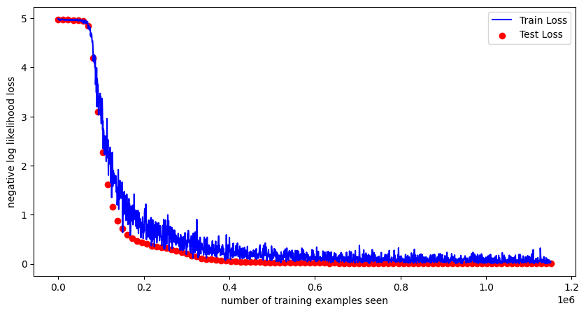
Let´s train for 100 epochs and see what results we get:

Test set: Avg. loss: 4.97100, Accuracy: 80/11520 (0.69%)

Train Epoch: 1 [0/11520 (0.00%)]	Loss: 4.98497
Train Epoch: 1 [640/11520 (5.56%)]	Loss: 4.97070
Train Epoch: 1 [1280/11520 (11.11%)]	Loss: 4.98385
Train Epoch: 1 [1920/11520 (16.67%)]	Loss: 4.97887
Train Epoch: 1 [2560/11520 (22.22%)]	Loss: 4.98134
Train Epoch: 1 [3200/11520 (27.78%)]	Loss: 4.95740
Train Epoch: 1 [3840/11520 (33.33%)]	Loss: 4.96550
Train Epoch: 1 [4480/11520 (38.89%)]	Loss: 4.96312
Train Epoch: 1 [5120/11520 (44.44%)]	Loss: 4.97780
Train Epoch: 1 [5760/11520 (50.00%)]	Loss: 4.96539
Train Epoch: 1 [6400/11520 (55.56%)]	Loss: 4.97644
Train Epoch: 1 [7040/11520 (61.11%)]	Loss: 4.97988
Train Epoch: 1 [7680/11520 (66.67%)]	Loss: 4.97382
Train Epoch: 1 [8320/11520 (72.22%)]	Loss: 4.97541
Train Epoch: 1 [8960/11520 (77.78%)]	Loss: 4.96909
Train Epoch: 1 [9600/11520 (83.33%)]	Loss: 4.97213
Train Epoch: 1 [10240/11520 (88.89%)]	Loss: 4.98121
Train Epoch: 1 [10880/11520 (94.44%)]	Loss: 4.96982

Test set: Avg. loss: 4.96955, Accuracy: 147/11520 (1.28%)
...
...
...
Train Epoch: 100 [0/11520 (0.00%)]	Loss: 0.12292
Train Epoch: 100 [640/11520 (5.56%)]	Loss: 0.08896
Train Epoch: 100 [1280/11520 (11.11%)]	Loss: 0.05819
Train Epoch: 100 [1920/11520 (16.67%)]	Loss: 0.00860
Train Epoch: 100 [2560/11520 (22.22%)]	Loss: 0.09907
Train Epoch: 100 [3200/11520 (27.78%)]	Loss: 0.00490
Train Epoch: 100 [3840/11520 (33.33%)]	Loss: 0.00973
Train Epoch: 100 [4480/11520 (38.89%)]	Loss: 0.05211
Train Epoch: 100 [5120/11520 (44.44%)]	Loss: 0.02216
Train Epoch: 100 [5760/11520 (50.00%)]	Loss: 0.06890
Train Epoch: 100 [6400/11520 (55.56%)]	Loss: 0.08246
Train Epoch: 100 [7040/11520 (61.11%)]	Loss: 0.01433
Train Epoch: 100 [7680/11520 (66.67%)]	Loss: 0.04654
Train Epoch: 100 [8320/11520 (72.22%)]	Loss: 0.02989
Train Epoch: 100 [8960/11520 (77.78%)]	Loss: 0.04203
Train Epoch: 100 [9600/11520 (83.33%)]	Loss: 0.05725
Train Epoch: 100 [10240/11520 (88.89%)]	Loss: 0.01901
Train Epoch: 100 [10880/11520 (94.44%)]	Loss: 0.04729

Test set: Avg. loss: 0.00748, Accuracy: 11502/11520 (99.84%)

We achieve a 99.84% accuracy in our predictions on our test set! Isn’t it amazing that we are able to detect in almost every image the correct time? Of course we had a very clean dataset with a lot of already labeled images.

Lets show some detected samples:

fig = plt.figure(figsize=(10, 5))
plt.plot(train_counter, train_losses, color="blue")
plt.scatter(test_counter, test_losses, color="red")
plt.legend(["Train Loss", "Test Loss"], loc="upper right")
plt.xlabel("number of training examples seen")
plt.ylabel("negative log likelihood loss")
fig.show()

with torch.no_grad():
    output = network(example_data.to(device))

fig = plt.figure()
for i, random_num in enumerate([np.random.randint(1, 64) for x in range(6)]):
    plt.subplot(2, 3, i + 1)
    plt.tight_layout()
    # Permutation needed to add color again
    plt.imshow(
        example_data[random_num].permute(1, 2, 0), cmap="gray", interpolation="none"
    )
    plt.title(
        f"Prediction: {time_dict[output.data.max(1, keepdim=True)[1][random_num].item()]}"
    )
    plt.xticks([])
    plt.yticks([])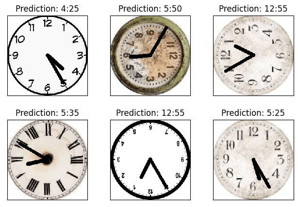

I think that will be all for now with classification models. Next step is to move into object detection, lets see what we can do there!

We will look at classification again in the future but it will be mostly in full project applications.

Find all the code at GitHub