
Recently I wanted to build a Neural Network from scratch as an exercise to work on the math behind neural networks and also to show that it is relatively easy to create networks in python just using the NumPy module. As a step 2 and in future posts I will continue building up on this knowledge, by showing how to build simple (and later more complex) Neural Networks with the well-known and existing frameworks Pytorch and Tensorflow.
I will use Python as the programming language and many online references that you can find in the reference list of my GitHub repo. There is already great work out there regarding this topic.
Neural Networks
I assume that the reader has some basic knowledge of what Neural Networks are, but just in case the definition from Wikipedia says:
Artificial neural networks, usually simply called neural networks or neural nets, are computing systems inspired by the biological neural networks that constitute animal brains. An ANN is based on a collection of connected units or nodes called artificial neurons, which loosely model the neurons in a biological brain.

The approach:
- The network receives input data
- Data moves through the layers (forward propagation)
- Calculate the error
- Backward propagation. We adjust the given parameters of our network.
Usually, it will be the derivative of our error with respect to the parameter - Iterate through that process, depending on the number of batches.
Programming of Basic Network
In this Medium post, there is a very good explanation of the mathematical principles behind neural nets and how to implement basic networks. I recommend the reader to follow the tutorial if you are interested in completely building a network from scratch. In my GitHub repository for this post, you can find my implementation of this blog with some code improvements, changes in the project structure also with some additional activation functions.
I would like to walk you through the Convolutional Neural Network implementation, as these are some of the most popular Deep Learning networks today, we will revisit these several times in the future when we apply them through well-known frameworks.
Convolutional Neural Network (CNN)
We will try two implementations of CNN one with two convolutional layers and one with just one layer. We will as well compare the results when using different types of activation functions.
The architecture of the convolutional layer looks the following way:

With Convolution Layers using the following code for forward and backward propagation:
class ConvolutionLayer(Layer):
    """
    A layer that uses convolution, based on math from
    https://medium.com/@2017csm1006/forward-and-backpropagation-in-convolutional-
    neural-network-4dfa96d7b37e

    Attributes:
    - input_shape = (i,j,d)
    - kernel_shape = (m,n) size of filter
    - layer_depth = output_depth

    Methods:
    - forward_propagation
    - backward_propagation
    """

    def __init__(
        self,
        input_shape: tuple[tuple[int], tuple[int], int],
        kernel_shape: tuple[int],
        layer_depth: int,
    ) -> None:
        self.input_shape = input_shape
        self.input_depth = input_shape[2]
        self.kernel_shape = kernel_shape
        self.layer_depth = layer_depth
        self.output_shape = (
            input_shape[0] - kernel_shape[0] + 1,
            input_shape[1] - kernel_shape[1] + 1,
            layer_depth,
        )
        self.weights = (
            np.random.rand(
                kernel_shape[0], kernel_shape[1], self.input_depth, layer_depth
            )
            - 0.5
        )
        self.bias = np.random.rand(layer_depth) - 0.5

    def forward_propagation(self, input: np.ndarray[float]) -> np.ndarray[float]:
        self.input = input
        # initialize output to zero
        self.output = np.zeros(self.output_shape)
        for k in range(self.layer_depth):
            for d in range(self.input_depth):
                # use np convolve with valid to not have the zero padding
                self.output[:, :, k] += (
                    signal.correlate2d(
                        self.input[:, :, d], self.weights[:, :, d, k], "valid"
                    )
                    + self.bias[k]
                )
        return self.output

    #
    def backward_propagation(
        self, output_error: np.ndarray[float], learning_rate: float
    ) -> np.ndarray[float]:
        """
        Calculates errors and backprop dE/dW, dE/dB, dE/dY, input error=dE/dX
        """
        in_error = np.zeros(self.input_shape)
        dWeights = np.zeros(
            (
                self.kernel_shape[0],
                self.kernel_shape[1],
                self.input_depth,
                self.layer_depth,
            )
        )
        dBias = np.zeros(self.layer_depth)

        for k in range(self.layer_depth):
            for d in range(self.input_depth):
                in_error[:, :, d] += signal.convolve2d(
                    output_error[:, :, k], self.weights[:, :, d, k], "full"
                )
                dWeights[:, :, d, k] = signal.correlate2d(
                    self.input[:, :, d], output_error[:, :, k], "valid"
                )
                dBias[k] = self.layer_depth * np.sum(output_error[:, :, k])

                self.weights -= learning_rate * dWeights
                self.bias -= learning_rate * dBias
        return in_error
As activation functions, we will use tanh for all the layers except the output where we will use Softmax. The implementation of tanh is very straightforward. We will need the tanh for the forward propagation of our network and the derivative of tanh for the backward propagation. Why tanh? The reason for adding this as an activation function is to add non-linearity to our layers, it has shown quite good results as an activation function for multi-layer networks.
def tanh(x: np.ndarray[float]) -> np.ndarray[float]:
    return np.tanh(x)


def tanh_prime(x: np.ndarray[float]) -> np.ndarray[float]:
    # print("tanh", (1 - np.tanh(x) ** 2).shape)
    return 1 - np.tanh(x) ** 2
The other activation function that we will use and the one that is generally chosen for the output layer is a generalization of the logistic function (sigmoid) for several dimensions. It is a bit more complex to program, and there have been also many articles written on how to implement this function in python. I have based my implementation on this Medium article. We also build a filter for vectorized or non-vectorized inputs.
def softmax(x: np.ndarray[float]) -> np.ndarray[float]:
    e = np.exp(x)
    return e / np.sum(e, axis=1)


def softmax_prime(x: np.ndarray[float]) -> np.ndarray[float]:
    """
    Returns the derivative of the softmax. Filters depending on if the input is
    vectorized or not
    """
    if x.shape[0] == 1:
        # Reshape the 1-d softmax to 2-d so that np.dot will do the matrix mult
        s = softmax(x)
        s = s.reshape(-1, 1)
        # Use the diagonal to return the values in the shape we need them for
          backprop
        return np.diagonal(np.diagflat(s) - np.dot(s, s.T))

    else:
        # input s is softmax value of the original input x.
        # s.shape = (1, n)
        # i.e. s = np.array([0.3, 0.7]), x = np.array([0, 1])

        s = softmax(x)
        # initialize the 2-D jacobian matrix.
        jacobian_m = np.diag(s)
        for i in range(len(jacobian_m)):
            for j in range(len(jacobian_m)):
                if i == j:
                    jacobian_m[i][j] = s[i] * (1 - s[i])
                else:
                    jacobian_m[i, j] = -s[i] * s[j]
        return jacobian_m
Results
We will test our network in the well know Mnist dataset. Check out the full code at GitHub. Remember to set your random seed to 0 if you want to reproduce the same results. Also for the loss function we have used Mean Square error, in later implementations we will also add the Cross-Entropy Loss.
from tensorflow.keras.datasets import mnist
from tensorflow.keras.utils import to_categorical

(x_train, y_train), (x_test, y_test) = mnist.load_data()

x_train, x_test = np.array(x_train, np.float32), np.array(x_test, np.float32)
# Flatten
x_train, x_test = x_train.reshape(x_train.shape[0], 28, 28, 1), x_test.reshape(
    x_test.shape[0], 28, 28, 1
)
x_train, x_test = x_train / 255, x_test / 255
print(x_train.shape, x_test.shape)

y_train = to_categorical(y_train)
y_test = to_categorical(y_test)
# Create CNN
cnn = Network()
cnn.add_layer(
    ConvolutionLayer((28, 28, 1), (3, 3), 1)
)  # input (28,28,1) output (26,26,1)
cnn.add_layer(ActivationLayer(tanh, tanh_prime))
cnn.add_layer(
    ConvolutionLayer((26, 26, 1), (3, 3), 1)
)  # input (26,26,1) output (24,24,1)
cnn.add_layer(ActivationLayer(tanh, tanh_prime))
cnn.add_layer(FlattenLayer())  # input (24,24,1) output (1,24*24*1)
cnn.add_layer(FCLayer(24 * 24 * 1, 100))  # input (1, 24*24*1) output (1,100)
cnn.add_layer(ActivationLayer(tanh, tanh_prime))
cnn.add_layer(FCLayer(100, 10))  # input (1,100) output (1,10)
cnn.add_layer(ActivationLayer(softmax, softmax_prime))

cnn.set_loss(mse, mse_prime)
cnn.fit(x_train[0:2000], y_train[0:2000], epochs=100, learning_rate=0.1)
We get amazing results for such a simple network of just 2 layers:
epoch98 / 100    error=0.0006699464787902453
epoch99 / 100    error=0.0006630306084486346
epoch100 / 100    error=0.0006546040013790374

Result:
[array([[2.47044493e-06, 5.55572747e-09, 7.39166242e-06, 3.80292561e-04,
        5.71749136e-07, 2.57341402e-04, 6.03182851e-11, 9.91674777e-01,
        1.35198090e-07, 7.67701406e-03]]), array([[9.14584799e-06, 1.48262122e-03, 9.92633433e-01, 2.05034219e-05,
        1.54224588e-07, 1.06154336e-03, 3.37702473e-03, 2.81653398e-08,
        1.41472300e-03, 8.23339559e-07]]), array([[4.59487233e-09, 9.91143919e-01, 4.62025182e-03, 7.61164053e-04,
        7.84496065e-05, 4.24055830e-04, 7.99882365e-05, 2.81081540e-03,
        7.66538372e-05, 4.69724760e-06]])]
true values:  [[0. 0. 0. 0. 0. 0. 0. 1. 0. 0.]
 [0. 0. 1. 0. 0. 0. 0. 0. 0. 0.]
 [0. 1. 0. 0. 0. 0. 0. 0. 0. 0.]]
Let us compare the errors of similar networks just to see the effects of different activation functions and or Network depth.
Only 1 convolution layer, keeping softmax for our output layer. We can see similar results, we achieve a bit better loss in the 2 convolution layer network.
epoch98 / 100    error=0.0008998702628854407
epoch99 / 100    error=0.0008919858380656314
epoch100 / 100    error=0.0008845053795560065
Only 1 convolution layer but using tanh as the activation function also for the output layer. We can see a significant drop in the loss function (2 orders of magnitude)
epoch98 / 100    error=0.045805609540409804
epoch99 / 100    error=0.04610471432050303
epoch100 / 100    error=0.04563577203218581
Let us see the effects of adding a second convolution layer to see if we can improve these results while keeping tanh as the output layer activation function. We can see a big reduction in the error due to the extra layer, but we are still 2 orders of magnitude higher than when we change our output layer activation function to the softmax.
epoch98 / 100    error=0.015739728961459264
epoch99 / 100    error=0.015656256249360245
epoch100 / 100    error=0.015574043589304339
Just to also consider the effect of the epochs in our results. In our last experiment, we obtain after 100 epochs a loss of 0.0156. For our best-performing model so far we achieved these results after just 6 epochs.
epoch5 / 100    error=0.01738538108832097
epoch6 / 100    error=0.014646911836040586
epoch7 / 100    error=0.012567932587293648
Summary of results:
| Convolution Layers | Filter size | FC Layers | Output Activation Function | Epochs | Loss |
| 2 | 3×3 | 2 | Softmax | 100 | 0.00065 |
| 2 | 3×3 | 2 | Tanh | 100 | 0.01557 |
| 1 | 3×3 | 2 | Softmax | 100 | 0.0008 |
| 1 | 3×3 | 2 | Tanh | 100 | 0.04563 |
Trying out our network in some test samples:
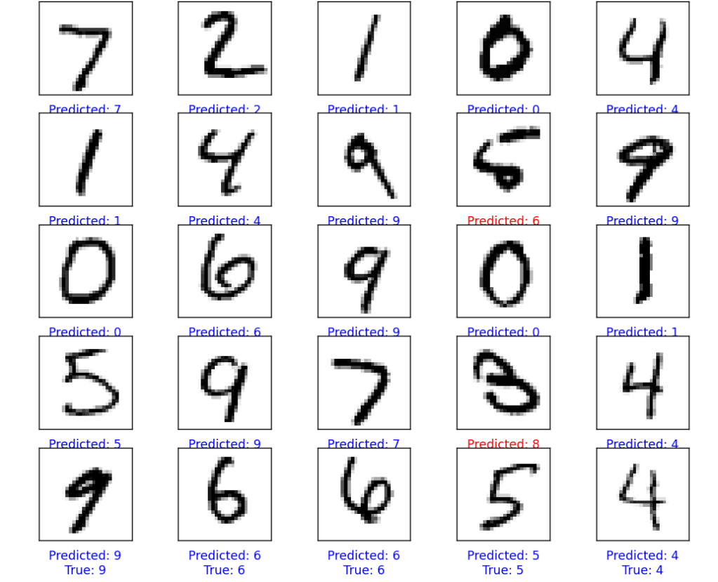
These results are very useful to understand how we can improve the result of our Network. In this case we see that the following factors improve our results greatly:
- Use Softmax as an activation function for the last layer
- Increase the number of convolution layers in the network.
Generally, for different applications you will focus on different network architecture aspects, depth of the network, activation functions to be used, and tuning of other hyperparameters that we will see in future posts.
If you are interested in following along and checking all the code for this post visit my GitHub.
Latest posts
- Transform Your Video Calls into Actionable Notion Notes with this AI assistant
- Revolutionizing Psychology Sessions with AI: Introducing Psycology Pal a Clinical Assistant App
- A journey through Neural Networks -part 3: It’s about time
- A journey through Neural Networks – part 2: how to PyTorch
- A journey through Neural Networks – part 1: Baby Steps

Leave a comment